The ‘Emotional’ Investor

“The purely economic man is indeed close to being a social moron. Economic theory has been much preoccupied with this rational fool.” — Richard Thaler, Misbehaving

We are taught that taking risks, despite the suffering that may come with them, reaps the greatest rewards. Society pushes us to “start that business”, “stand up for that cause”, or even “ask that person out on a date”. Risk fundamentally drives progress.

It is no different in financial markets. You probably know the saying “high risk, high return”. This risk-return trade-off lays the foundation for arguably the most important model in financial history, the Capital Asset Pricing Model (CAPM):

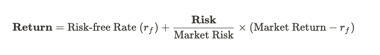
However, this whole model makes one vital mistake: it assumes people are rational, or, as Thaler says, “social morons”.

In reality, we make mistakes. We get scared and can be overconfident. All that emotion deeply changes how we think and make decisions. It’s not that the CAPM is useless, but the truth is far more complex and nuanced.

The 2021 paper, ‘Prospect Theory and Stock Market Anomalies’, gives 23 different examples of how the CAPM fails, calling these ‘stock market anomalies’. An interesting example is the ‘momentum anomaly’: stocks with great past returns tend to outperform the CAPM, whilst stocks with poor past returns tend to underperform the CAPM.

Clearly, the CAPM does not suffice. We need a new and improved model, one that accounts for our ‘emotional’ investor. Three economists from Yale, Caltech and Florida have done just that.

It turns out, their psychological model successfully predicts most of these anomalies. A huge improvement on the CAPM. This begs the question, should hedge fund managers be going to their shrink for investment advice?

So, what is this psychological model?

This paper builds upon prospect theory, a psychological model which won one of its creators, Daniel Kahneman, the 2002 Nobel Prize in Economics and sparked the birth of behavioural economics. It introduces three key behaviours people have when making risky decisions:

Loss aversion describes how we are affected more by loss of wealth than gains. Finding $50 on the street is nice, but losing $50 REALLY sucks (maybe not for Jeff Bezos though).
Diminishing sensitivity means we are affected less and less by changes in wealth the further we are from our initial wealth. Losing $10 sucks, but losing another $10 an hour later isn’t as bad.
Probability weighting refers to our consistent overweighting of highly unlikely events and underweighting of highly likely events when making decisions. If you’ve ever asked yourself, “why is everyone so afraid of the AstraZeneca vaccine?” or “why does everyone believe they’ve got a shot at winning the lottery?”, the answer: probability weighting.

The first two of these phenomena can be seen in the value function below; the third in the weighting function. Note, x is the total change in wealth and P is the probability of some event occurring.

First, the value function is steeper for x < 0 as losses are felt more than gains. Second, the value function gets flatter as you move from x = 0 in either direction, due to diminishing sensitivity. Third, the inverse S-shaped weighting curves (red and blue) illustrate the over and underweighting described by probability weighting.

What does this mean for investors?

Put simply; loss aversion means we find volatility unattractive. To be compensated for this unattractive volatility, investors require a higher rate of return. Yes, this is the same prediction as the CAPM. But this time, the model doesn’t stop there…

Diminishing sensitivity means we are more willing to take on risks after losing money and less willing after gaining money. Hence, if an investment has lost money in the past, we require a lower return on it in the future. On the other hand, we require a higher return on investments that have made money in the past. The paper calls these past gains (or losses) the capital gain overhang of the stock.

The consequence of probability weighting is that we are disproportionately affected by the tails of return distributions. Therefore, we find positively skewed (long right-tailed) return distributions attractive and hence require a lower return on assets with such distributions.

Can psychology explain the market?

To answer this question, the authors of this paper transform prospect theory into a quantitative model in order to make numerical predictions about stock returns.

For all you maths nerds out there, they first build a value function and a probability weighting function (like above). Essentially, they integrate a stock’s return distribution over these two functions to develop a model predicted return. If you didn’t understand a word we just said, don’t worry. The rest of the analysis is far easier to grasp.

The paper compares the historical returns of US stocks with the returns predicted by their psychological model. In the graphs below, we show the results for four anomalies the model predicts well. Blue indicates the return predicted by the model; orange is the observed return from the data.

As stock market anomalies refer to incorrect CAPM predictions, it makes sense to quote the model and observed returns in terms of **alpha** (the difference between the model/observed return and the CAPM predicted return)

Notice how close those lines are to each other?

Now, let’s zoom in on the momentum anomaly. We said earlier that stocks with high momentum tend to have positive alpha whilst stocks with low or negative momentum tend to have negative alpha. Higher decile stocks (the ones with the highest momentum) are less volatile than their lower momentum counterparts. However, these stocks are also more negatively skewed and have a larger capital gain overhang than their lower momentum counterparts.

As it turns out, the latter force dominates, causing the model to match the data, where higher momentum stocks outperform the CAPM and lower momentum stocks underperform the CAPM.

In the end, the prospect theory model matches the data for 14 of the 23 anomalies it attempts to predict. In other words, it solves ~60% of the mistakes the CAPM makes. So, can psychology help explain the market? The simple answer to our question is alarmingly, yes.

What can’t the psychologist explain?

You might be thinking, “what about the other nine anomalies the model doesn’t explain?”. The paper argues the impact of prospect theory on such anomalies still exists, but other factors swamp it.

In fact, they show for five of those nine, the anomaly only materialises around earnings announcements. This suggests these anomalies are largely due to investors’ incorrect beliefs about firms’ prospects — which are then corrected by earnings releases. The authors argue,

“This, in turn, raises the possibility that many anomalies can be put into one of two categories: ‘preference-based’ anomalies that are driven by risk attitudes of the kind captured by prospect theory and ‘belief-based’ anomalies that are driven by incorrect beliefs.”

Whilst this paper doesn’t attempt to explain these ‘belief-based’ anomalies, it makes huge strides in explaining the ‘preference-based’ anomalies.

How do we use this?

When you’re making an investment, don’t think there’s some quantitative genius on the other side of the trade.

In reality, they’re just like all of us.

They have their limitations and their biases. They aren’t like Benjamin Graham’s ‘intelligent investor’. They are ‘emotional’ investors as much as you or me.

A more detailed discussion (Additional reading)

This is an extra section to the articles at the end to explain any simplifications we made, discuss more intricately complex parts of the paper and introduce any extra thoughts we have on the academic implications of the work.

The value function given in our article has formula:

x is just the gain or loss in wealth from some event.
Here, α is strictly between 0 and 1. This ensures the curve is concave for gains and convex for losses. A higher α constitutes weaker diminishing sensitivity. From previous studies into the risk appetites of the general population and that of financial professionals, the paper assumes α to be 0.7.
λ is greater than 1, therefore representing loss aversion. The higher the value of λ, the more loss averse the agent is. This paper assumes λ to be 1.5.

The probability weighting function given in the article has the formula:

w(P) is the weighting we give to a specific probability P. To understand this, have a think about overweighting small probabilities in the case of a lottery. If the true probability you win the lottery is one in a million, P is one in a million. However, when you are making a decision to buy a lottery ticket, you may subconsciously overweight this probability. Hence, w(P) could be one in ten-thousand.
δ quantifies the level of over/under weighting and is between 0 and 1. Higher δ represents higher mis-weighting. This paper assumes it to be 0.65.

Each investor’s maximisation problem is given by the objective function:

The δ’s are the weights given to each risky asset 1,…,N.
E(W_1) is the expected value of wealth in the future period t=1.
Var(W_1) is the variance of future wealth. The first two terms in this objective function represent traditional mean-variance preferences (just like the CAPM). γ is the level of volatility aversion for the investor.
b_0 is the weighting given to prospect theory. G_i is the future gain or loss on the asset plus the past gain or loss on the asset. V(G_i) gives the cumulative value for such a G_i, given prospect theory.

For those of you who are super keen, here is V(G_i):

P(R_i) is the probability distribution of returns. It is later assumed to be the “generalised hyperbolic (GH) skewed t distribution”, a distribution especially effective at modelling skewness.
The top term refers to losses and the bottom refers to gains, hence the λ out the front of the top term.

The model assumes an equilibrium structure they call “bounded rationality with heterogeneous holding”. Have a look at the paper if you want to know this in detail, it is quite challenging…

Essentially, there are a few parameters underlying the returns distribution. The authors input such parameters in order to match the historical data on the volatility, skewness and beta of the empirical returns distribution. Finally, they derive a model predicted return that clears the market given the equilibrium set-up.

The rule they adopt for determining whether or not the model explains an anomaly is as follows:

First, from the data, they rank all stocks by their exposure to some anomaly. For example, they rank all stocks from most momentum to least momentum. They then split them into deciles. They do the same for the stocks produced by the model.
They then conclude the model explains the anomaly if the following two conditions are met:

α^d is the empirical alpha for some decile; α^m is the model predicted α for some decile.
To say the model predicts the anomaly, the model must accurately predict the direction of the anomaly moving from decile 1 to decile 10, and the difference in predicted α for both deciles must be large enough to constitute a significant prediction.
The model performs better than the CAPM and the Fama-French 3 factor model, similarly to the Carhart 4 factor model and worse than the Fama-French 5 and 6 factor models. However, the factor models are all derived with the anomalies in mind, whereas this model is derived only from the risk attitudes of investors.